Neuronal detection of social actions directs collective escape behaviour – Nature

Fish husbandry

D. cerebrum^{13,14,15,33,35,54,60,61,62,63} were raised and maintained in conventional zebrafish housing systems (Aquaneering; system water temperature 29 ± 0.5 °C, pH 7.0, conductivity 600 µS cm⁻¹), under 14:10 h light:dark cycles, and were fed 2–3 times a day. D. cerebrum were bred in communal tanks of ~40–60 individuals, enriched with ~5 cm silicone tubes to encourage spawning. Eggs were collected during the first 1 h of daylight, and 1–2 h after morning and afternoon feeding. Embryos (0–5 days post-fertilization (dpf)) were raised in egg-water (5 mM NaCl, 169 μM KCl, 330 μM CaCl₂, 161 μM MgSO₄∙7H₂O, and 0.15% methylene blue dissolved in reverse osmosis purified water) in an incubator at 29 ± 0.5 °C.

Larvae (5–14 dpf) were housed in static tanks in the housing systems and cocultured with L-type rotifers (Brachionus plicatilis), while water level was raised ~1 cm per day. At 21 dpf, the housing tank was connected to the water circulation system and fish were fed with artemia. At 8–10 weeks post-fertilization, D. cerebrum reach adulthood and become fertile. Wild-type D. cerebrum were provided by A. Douglass and B. Judkewitz. The transgenic line Tg(elavl3:H2B-GCaMP6s)⁶⁴ was provided by B. Judkewitz.

The behavioural and imaging experiments with D. cerebrum were approved by the government authorities (US Animal Care, and Institutional Animal Care and Use Committee (IACUC), (USDA Registration Number 93-R-0437)) and carried out in accordance with the US federal and California state law to enforce the Animal Welfare Act (AWA) under the California Health and Safety Code.

Behavioural experiments setups

All behavioural experiments used D. cerebrum that were at least 8 weeks old, and included both sexes. Behavioural recordings were conducted in a room with a portable electric heater to maintain water temperature between 28–30 °C. Data acquisition was automated and timestamped in BonsaiRx^65,66 ( All behavioural arenas were built with custom cut acrylic (black walls and transparent bottom with white styrene to diffuse bottom lit light sources) and encircled with black curtain to control luminance. Light and dark environments are controlled with a bottom-projected white or dark background (AnyBeam Pico Projector, HD301M1-H2).

Behaviours were illuminated with infrared light (CM-IR130-850NM, CMVision Technologies) from the bottom, and acquired at 121 Hz from a camera mounted above (FLIR Grasshopper, 33-534) with an 8 mm/F1.8 lens (Edmund Optics, 15-626) and long-pass filter (Edmund Optics, 12-767).

Behavioural tracking and processing

Social LEAP-Estimates Animal Poses (SLEAP)⁶⁷ was used to train models for tracking the location and posture of D. cerebrum. Each video was proofread after inference and identity tracking to create h5 files that contain positional information of all tracking nodes of each animal for the given behavioural session. The h5 files and a corresponding timestamped csv were processed with custom Python code (3.12) for further analysis (see Code availability). Models were trained with a nine-node skeleton covering the two eyes and evenly distributed points along the midline of the body and tail.

For each time point, animal centroid was defined as the xy coordinates of the middle point of the two lobes of the swim bladder. A nose point was defined as the centre point of the 2 eyes, and the orientation of the animal was defined as the direction of the vector pointing from the centroid to the nose point and smoothed by a 5-frame running average (~40 ms). Speed and angular speed of the animal was calculated by taking the derivatives of centroid coordinates and the heading direction and smoothed by a 10-frame running average (~80 ms), respectively. Distance and alignment of each fish to all its neighbours were identified for each time point. All x and y coordinates were then transformed from pixel to mm by measuring the arena edge, a known physical length, in Fiji. We saved csv files with the timestamps for each video frame and any stimulus presented. Python code aligned all arrays to the behaviour before further analysis.

Visual loom-evoked escape assay

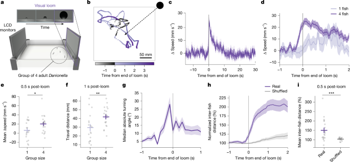
In the loom-evoked escape behaviours, D. cerebrum were left to habituate for 20 min in a square arena (265 × 265 mm) where two of the walls were lined with 10.1-inch LCD monitors (HAMTYSAN, 10.1 inch rendered at 1,024 × 600 pix). Each screen was mapped as a 14 × 20 cm window into a 3D virtual environment, eye perspective at centre point of area, 2 cm above the bottom, using BonVision package⁶⁶. Each experiment consisted of 5× 2-min recordings, and at the 1-min mark a dark sphere of 4.3 cm would appear in one of the corners (x = ±30, y = ±15, z = 1.5 cm) (Extended Data Fig. 1b) and move linearly to the centre of the arena (x = 0, y = 0, z = 1.5 cm) within 3–6 s. With a total virtual displacement of 33.5 cm, the loom moved at a constant speed of 5.6–11.2 cm s⁻¹, creating a length/velocity (L/V) ratio ranging from 384 to 769 ms. Both the starting position and moving duration were randomly determined. We separated each trial by 5-min intervals and used groups of 1, 2, 4 and 8 fish.

Baseline swimming speed in the 30 s before loom onset was fitted with Gaussian mixture model with four Gaussian components (determined by Bayesian information criterion) for single fish and fish in a group of four separately (Extended Data Fig. 1e). The boundary between the second and third components was defined as the threshold between low and high swimming speed. We defined escape latency as the first time point when a fish reached high speed if that time event occurred within 1 s after the end of loom (Extended Data Fig. 1f). We calculated the change in speed from looming stimulus by normalizing each fish’s speed 0.5 s after the end the stimulus to its mean speed 30 s prior to the onset of the loom (Fig. 1d,e). Travel distance before and after stimulus was calculated with integration of speed over 1 s (Fig. 1f and Extended Data Fig. 1g,l,m) window.

Turning behaviour was calculated by taking the absolute heading direction changes in 0.05-s bins, and plot it as probability density function (PDF) or cumulative distribution function over continuous 250-ms block (Extended Data Fig. 1n,o). Same statistical curves were plotted with 100-ms blocks to visualize the median turning angles (Fig. 1g). Inter-fish distance was calculated for each pair of fish within a group. The positions of each fish in the group were shifted by a random number independently to create the shuffled data used to calculate temporally shuffled inter-fish distance (Fig. 1h), and the trajectories of all fish were shuffled post end of loom to create chance level of spatially shuffled inter-fish distance (Extended Data Fig. 1r). Change in inter-fish distance was computed by subtracting the mean over 1 s before loom onset, and the mean at 0.5 s after the stimulus are used for statistical comparison (Fig. 1i).

Eye angle tracing of the loom was performed via two-dimensional ray-casting. In each video frame during loom stimulus presentation, we calculated the coordinates of the virtual sphere, and drew angles from the fish’s midpoint (between the two eyes) to the edges of the 4.3 cm sphere. The angular size of the loom is the absolute angle difference between the vectors to the left and right side of the sphere (Fig. 2a,b, Extended Data Fig. 4a,b). Speed from 6 s before the threshold was used as baseline to calculate changes (Fig. 2b,c).

We created Boolean arrays to identify when each fish first senses the loom at the threshold angle of 7°. These arrays were resampled to align trials of different lengths (speeds of 5.6–11.2 cm s⁻¹), and construct the cumulative probability curve of reaching loom threshold (Fig. 2e and Extended Data Fig. 4b). Using trials aligned from loom start to loom end, we identified the time through the trial where 50% of group members pass the angle threshold. This time point was used to assign individual and group information status in the subsequent analysis. For individuals, they were labelled as ‘early-informed’ if loom reaches critical angle at an earlier time than this cut-off. Otherwise, individuals were labelled as ‘late-informed’, including those that never reached critical angles and did not have a valid reaching time (that is, the angle of the loom never reached 7°). The mean of the threshold-reaching time in a group was also compared to the same cut-off to assign the group as ‘early group’ or ‘late group’ (Fig. 2e). Therefore, early groups contained more early-informed individuals, and vice versa. To compare behaviour across trials, we calculated the average speed in time bins 5% of the original trial length.

Mechanosensory tap-evoked escape assay

In the tap-evoked escape behaviours, D. cerebrum were left to habituate for 20 min prior to the experiment in a 350 mm circular arena filled with 1 l of system water¹⁵. Each experiment consisted of 5 repetitions of 2-min recordings, where an actuator (Adafruit Industries, TAU0730TM-14) mounted beneath one corner of the arena was moved by a 300-ms voltage pulse that delivered a mechanical tap at the 1-min mark. Each trial was separated by 7 min, and experiments included groups of 1, 2, 4 or 8 fish. For the light–dark experiments of tap escape, groups of 1 or 4 fish from a different cohort were used. Behaviours were run with either a white or black background bottom projection.

Baseline swimming speed in the 30 s before tap onset was fitted with Gaussian mixture model with four Gaussian components (determined by Bayesian information criterion) for single fish and fish in groups of four separately (Extended Data Fig. 2g). The boundary between the second and third components defined the threshold between low and high swimming speed. Escape latency within 1 s after the end of tap was identified as the first time point when a fish reached high speed (Extended Data Fig. 2h). The mean speed in the 30 s prior to the tap was used as the baseline for each individual fish to calculate how their speed changed 0.5 s after the tap (Extended Data Fig. 2d,e). Travel distance before and after the stimulus was calculated by integrating the speed over a 1 s (Extended Data Fig. 3d,e,i,j) window.

Turning behaviour was calculated by taking the absolute heading direction changes in 0.05-s bins, and plot it as PDF or cumulative distribution function over continuous 250-ms block (Extended Data Fig. 2n,o). Same statistical curves were plotted with 100-ms blocks to visualize the median turning angles (Extended Data Fig. 2p).

Inter-fish distance was calculated for each pair of fish within a group. The positions of each fish in the group were shifted by a random number independently to create the shuffled data used to calculate temporally shuffled inter-fish distance (Extended Data Fig. 2i,k), and the trajectories of all fish were shuffled post end of tap to create chance level of spatially shuffled inter-fish distance (Extended Data Fig. 2m). Change in inter-fish distance was computed by subtracting the mean over 1 s before tap onset, and the mean at 0.5 s after the stimulus are used for statistical comparison (Extended Data Figs. 2j and 3l).

Virtual conspecifics engagement and social escape assay

We created a 3D virtual reality (VR) environment using Panda3D ( and populated it with five virtual male D. cerebrum (Extended Data Fig. 5a) modelled in Blender (v3.5.1). The Danionella model was adapted from an image in Kadobianskyi et al.⁵⁹. The VR scene was captured by a virtual camera positioned in VR space such that the virtual D. cerebrum appeared on the bottom third of the monitor. These virtual conspecifics appeared on a single monitor, with the opposing monitor displaying an empty background. Each VR D. cerebrum appeared ~12 mm in length on the display and had animated tail movements that coincided with the burst phase of their burst-and-glide kinematics (Extended Data Fig. 5b). The virtual school was programmed to swim along the width of the monitor by translating their x position in VR space, with small, random deviations in z to simulate slight changes in depth. The school always remained in the field of view of the VR camera, and therefore appeared on the monitor, as each fish executed a 180° turn when they reached the boundary of environment.

The environment was rendered on the monitors of the same square arena used in loom-evoked escape assay (Fig. 3a). To establish whether the sight of our virtual school attracted real fish, we first implemented an open loop paradigm (Fig. 3b,c). Here, a single D. cerebrum was left to habituate for 5 min in a square arena before being shown 4× 5-min no stimulus followed by 5-min stimulus on, with 5 swimming virtual D. cerebrum. At the end of each stimulus-on period, all virtual fish were assigned a random escape heading spanning 150° towards the orientation of the virtual camera so they rapidly swam away from the virtual camera into the horizon of the VR environment (Fig. 3d). These actions were not contingent on the position of the real fish with respect to the virtual fish.

For the social escape assays, we implemented a closed-loop paradigm wherein the proximity of the real fish to the virtual school triggered an escape. For this, we again allowed a single D. cerebrum to habituate to the environment for 5 min. After 1 min of the 5-fish virtual school being displayed on the monitor, the test fish’s engagement with the virtual school (test fish distance to centre of virtual school <16 mm) triggered either an escape or disappearance of VR fish depending on the experiment (Figs. 3d,e and 5k and Extended Data Fig. 5c). The overhead camera served to track the centroid position of the fish in real time using the KNN background subtractor function from the openCV library. The number of escaping or disappearing virtual fish was randomized for experiments with differing numbers of escapees, with each fish experiencing a 1-, 3- and 5-fish-escape event from the group of 5 total in the school (Fig. 3f,g). Each trial was separated by 60 s wherein we displayed an empty background after the escape. The virtual fish then re-appeared on the screen and the process repeated for a total of three trials per fish. For trials examining the response to linear movement of the virtual school, we programmed the virtual fish to move at the average velocity of a burst-glide cycle and removed the tail movement animation. In the case of disappearing fish, they vanished at the onset of ‘escape’. We used a similar closed-loop trigger to initiate a black looming stimulus that emerged from the centre of the virtual school (Extended Data Fig. 8n,o). The looming stimulus expanded hyperbolically over the span of 0.75 s, averaging 54° s⁻¹, to a final size of 50 mm on the LCD monitor.

Fish immobilization and holding chamber for in vivo two-photon calcium imaging

We modified the head-tethered preparation and holding chamber design from Zada et al. 2024¹⁵. In brief, adult D. cerebrum were transiently anaesthetized with tricaine (120 mg l⁻¹ MS-222 for 1–2 min) before they were removed from water and placed ventral side up on a 24 × 30 × 1 mm coverslip (12545B, Fisher Scientific). Two pieces of pre-cured SYLGARD wedges were fixed on the coverslip with UV-cured plastic (Bondic) to support the fish body from behind the eyes. 5–10% low-melting point agarose (UltraPureTM LMP Agarose, Invitrogen) was added to cover the body from swim bladder to the proximal tail, and on the side of head in front of the SYLGARD pieces. Another horizontal strip of UV-cured plastic was added to connect the coverslip and the agarose for more stability. Agarose from the side of the eyes, gills, and the tip of the tail were removed with a scalpel. Once all components were dried, the fish was placed back into a holding dish and ventilated with oxygenated water to ensure gill movement. Fish that recovered and showed spontaneous gill ventilation were then moved into the holding chamber under the two-photon microscope.

The triangular chamber was built from two monitors (HAMTYSAN, 7-inch 800 × 480 LCD). The two screens occupied ~260 ° of visual space in azimuth (130 ° each side, with ~10 ° gap in the front, and ~90 ° gap behind the fish), and ~105 ° of visual space in elevation (52.5 ° below and above). The chamber was filled with fish housing water (28 °C, ~500 ml). The water level was maintained ~1 cm above the midline of monitor height (10 cm) by gravity flow of fresh fish housing water and a custom vacuum made from a bent borosilicate electrode (WPI) constantly removing excess water throughout the duration of the experiment.

The back wall and floors were made of transparent acrylic for IR lights and recording camera access. A 4.5 mm column of clear acrylic was used as a pedestal to position head-fixed fish at a standard positioning within this arena (intersection of each screen’s midpoint). Coverslips were suspended from the acrylic pedestal using two 3 ×1 mm magnets (Ethcool) that was embedded into the top of the pedestal and another one added when anchored.

Visual stimuli

Dot stimuli

BonsaiRx was used to record the timing of microscope frame acquisitions, and display visual stimuli. Visual stimuli were displayed on the screens using cube mapping in BonVision⁶⁶, where each screen displayed a viewport in a virtual environment. The virtual environment was composed of a 6,000 mm² plane with a smoothed white-noise pattern (‘seafloor’). The fish’s position in this VR world was in the centre (0,0 in xy coordinates), 10 mm above the seafloor.

For nonsocial stimuli, a dark sphere was programmed to appear in the front of fish in the virtual environment. After 1 s, it either moved horizontally to the periphery (linear motion stimulus) or moved toward the virtual camera (thus, expanding in size; loom stimulus) over 5 s (Extended Data Fig. 6b). For the social stimuli, behavioural recordings of swimming and escaping D. cerebrum from both top-down and lateral view were processed to obtain realistic position changes of fish in 3D space (Extended Data Fig. 6a). Behaviour tracking (121 and 200 Hz for the top-down and lateral side view) was resampled to the refresh rate of monitors (60 Hz) and applied to spheres. The diameter and distance of the spheres in the virtual environment were calibrated to match their size with live fish. The two smaller dots swam from the back to front of the head-tethered fish in the VR environment over 6 s (swim stimulus) or executed a downward and outward escape at the 3 s mark and kept swimming farther (Fig. 4d and Extended Data Fig. 6a,b). All stimuli within a session were delivered to one visual field (left or right).

Virtual D. cerebrum stimuli

A custom Python script was used to record the timing of microscope frame acquisitions and display visual stimuli. To simulate the presence of conspecifics, we constructed a 3D environment using Panda3D, positioning two virtual cameras to match the perspective of the head-tethered fish. A virtual school comprising three D. cerebrum were used, populating one visual field (left or right).

For stimulus types with biological motion, the virtual school moved with realistic burst-and-glide kinematics (rapidly accelerating and then exponentially decelerating at ~1 Hz, Extended Data Fig. 5b) and with animated tail movements that corresponded with the burst phase of motion. For stimulus types with linear motion, the virtual school moved with a constant velocity and without animated tail movements. The start and end position of each fish, as well as the average speed, were matched to stimuli swimming with biological motion. Movement in each trial lasted for 5 s, which corresponded to 4 burst-glide cycles, and was followed by either an escape or disappearance of the virtual fish, or the emergence of a looming stimulus. Escape trajectories spanned 45–135° away from the heading of the head-tethered fish. That is, the virtual fish veered to the left when they were displayed on the left screen, and they veered to the right when displayed on the right screen. To avoid contaminating our imaging path with green/blue light from the visual display, we lined the LCD monitors with red gel light filters (LILIYA, 8.5 × 11 inch cut to size) and red-shifted the virtual environment rendering with a graphic shader (Background colour is set as Light Coral (hex code f08080); ambient light RGB set to 1/0.5/0.5 to bias the light reflection from the seafloor and objects toward longer wavelength).

For both experiments, each recording session started with a 1–2 min baseline with only the seafloor background scene visible. We then used a trial structure to present each of the stimulus types to head-tethered fish for 10 trials each in a pseudorandomized order, with randomized 14–16 s inter-trial intervals. All stimuli were displayed underneath the water surface of the recording arena and on the same side of the monitor within the recording session (15–20 min). Concurrently, we recorded the tails of these fish using a FLIR Grasshopper camera (33-534) affixed with a long-pass filter (Edmund Optics, 12-767) at 30–120 Hz. Each video frame was also timestamped by the Bonsai or Python script for post hoc data synchronization.

Two-photon calcium imaging

Two-photon microscopy was performed with a ThorLabs Bergamo II multiphoton microscope controlled by ThorImageLS 4.3 and illuminated by an fs-pulsed 80-MHz Ti:S laser (MaiTai DeepSee; SpectraPhysics). GCaMP6s fluorescence was imaged with a 16×/0.8 W Nikon objective at an excitation wavelength of 930 nm and ≤10 mW excitation power. Frames of 1,024 × 1,024 pixels covered a field-of-view of 978 × 978 μm.

We imaged fish at a diagonal, to include as much of the brain in our field of view as possible^15,18. Depth of the imaging plane was determined by maximizing the number of cells in the optic tectum within the field of view. Dual-plane or single-plane imaging sessions were conducted for each fish if it maintained healthy spontaneous movement for the entirety of the experiments, where the stimuli came from each side of the visual field twice each. For two-plane imaging, we used fast z mode in ThorImageLS 4.3 to move across 50–90 μm at 5 Hz. For the single-plane imaging, a 2–3 frame average was used to produce a final effective imaging rate at 5–7.6 Hz.

Imaging analysis

We only proceeded with experiments where fish remained healthy at the end of recording and did not have substantial z-movements or drift during recording. For sessions with detected shifts in z, we trimmed the z-shifted frames if the remaining uncorrupted experimental length was more than half of the original time series, and analysed neural activity in this epoch.

Imaging data were motion corrected in Suite2p⁶⁸, followed by cell extraction. Time series were inspected using Rastermap⁶⁹ to ensure there was no z-motion contamination or slow drift, and we only included neurons with continuous measurements and which were classified as a cell by Suite2p (“iscell”=1). A cellpose⁷⁰ classifier was trained for cell extraction. The anatomical region where each neuron is located was further classified with manually defined boundaries; cells outside these boundaries were not included for region-specific analyses. We excluded the first 5% of each imaging trial to avoid the influence of sound-evoked activity upon the initiation of scanning. Stimulus timing and calcium traces were aligned and resampled to a common 10 Hz sampling rate for further analysis. Then the fluorescence traces were detrended, smoothed with a 1-s rolling mean, and z-scored. The z-scored fluorescence and the median xy coordinates for each cell within these boundaries were used for further analysis.

We identified stimulus-responsive cells by conducting a t-test between the mean z-scored fluorescence during the 6-s stimulus and the mean z-scored fluorescence in the 5-s baseline pre-stimulus. Neurons were identified as responsive to a certain stimulus type if the significance is P < 0.05. Offset cells are defined by peak response time (1) at or later than 6 s to biological motion (BM) stimulus onset and (2) between 3 and 6 s to BM-escape onset. Among them, those peaked at or later than 6 s to the linear stimulus onset are categorized as general-offset cells, and those peaked before 6 s are categorized as social-offset cells. For the support vector machine (SVM) models, we only used experiments where there were at least 8 trials for all four stimulus types. The decoders were trained on the principal components (those that explain 90% of variance) of neural activity from all responsive cells in each recording session. For longer sessions, 8 trials were randomly selected for each stimulus type and split with a stratified K-fold cross-validator (eightfold). Twenty-five iterations of training and testing were performed.

Tail motion was assessed by measuring the number of pixels corresponding to tail movement in each video frame during imaging sessions. We processed each video frame using three consecutive functions from the OpenCV library: First, we applied a uniform Gaussian blur to each frame (cv2.GaussianBlur). Second, we dilated the resulting image (cv2.MORPH_OPEN). Third, we used the KNN background subtractor function to identify and sum moving foreground pixels that corresponded to the moving tail (cv2.createBackgroundSubtractorKNN). To compare movement across videos, we z-scored the tail movement of each video comparing each frame to a 15 s rolling mean. Time points with a z-score exceeding 2 were classified as motion. We averaged significant movement across fish using a 500-ms bin, and each trial was categorized as a motion trial if the mean of significance movement during stimulus presentation exceeds zero.

Statistics

Groups were tested for normality using the Shapiro–Wilk test. Non-parametric tests (Mann–Whitney U, Kruskal–Wallis H) were conducted if the Shapiro–Wilk P < 0.05 for any group. Otherwise, parametric tests were used. Post hoc tests were conducted if main effect was P < 0.05. All post hoc tests (Dunn’s test for non-parametric data, or t-tests for parametric data) were corrected for multiple comparisons with a Bonferroni or Holm correction. For nested data (neurons within imaging session within experimental groups), we determined the significance of pairwise comparisons using linear mixed-effects models, with imaging session identity (id) as a random variable. Exact tests and P values are reported in Supplementary Table 1.